08. Lab: Encoder

FCN: Encoder

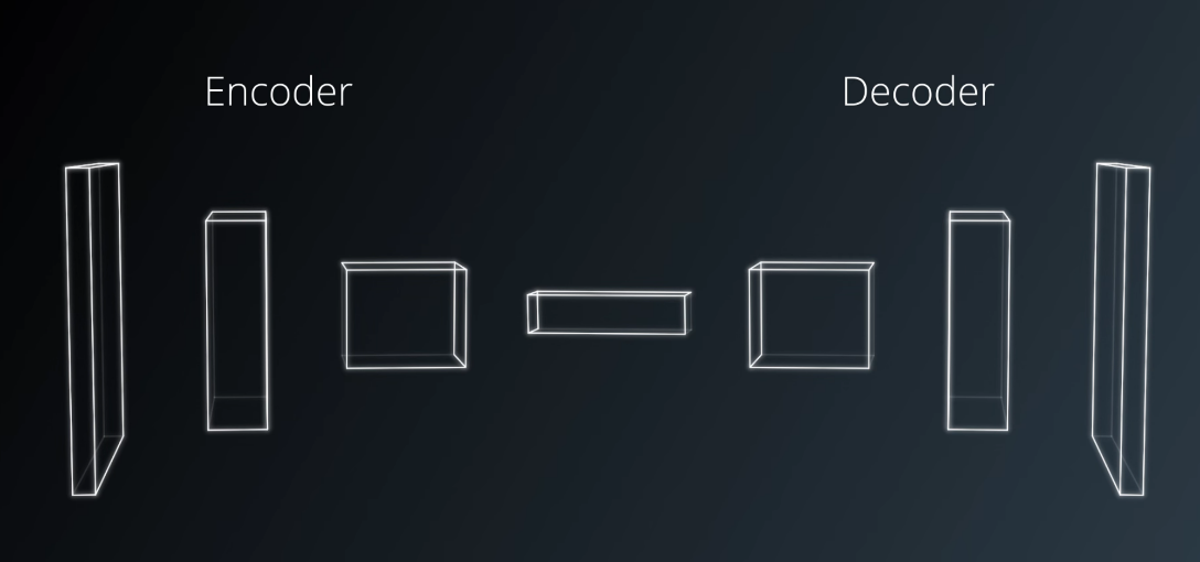
In the previous lesson, the FCN (Fully Convolutional Network) architecture was introduced. Recall that an FCN is comprised of an encoder and decoder. The encoder portion is a convolution network that reduces to a deeper 1x1 convolution layer, in contrast to a flat fully connected layer that would be used for basic classification of images. This difference has the effect of preserving spacial information from the image.

Separable Convolutions, introduced here, is a technique that reduces the number of parameters needed, thus increasing efficiency for the encoder network.

Separable Convolutions

Separable convolutions, also known as depthwise separable convolutions, comprise of a convolution performed over each channel of an input layer and followed by a 1x1 convolution that takes the output channels from the previous step and then combines them into an output layer.

This is different than regular convolutions that we covered before, mainly because of the reduction in the number of parameters. Let's consider a simple example.

Suppose we have an input shape of 32x32x3. With the desired number of 9 output channels and filters (kernels) of shape 3x3x3. In the regular convolutions, the 3 input channels get traversed by the 9 kernels. This would result in a total of 9*3*3*3 features (ignoring biases). That's a total of 243 parameters.

In case of the separable convolutions, the 3 input channels get traversed with 1 kernel each. That gives us 27 parameters (3*3*3) and 3 feature maps. In the next step, these 3 feature maps get traversed by 9 1x1 convolutions each. That results in a total of 27 (9*3) parameters. That's a total of 54 (27 + 27) parameters! Way less than the 243 parameters we got above. And as the size of the layers or channels increases, the difference will be more noticeable.

The reduction in the parameters make separable convolutions quite efficient with improved runtime performance and are also, as a result, useful for mobile applications. They also have the added benefit of reducing overfitting to an extent, because of the fewer parameters.

Additional Resources

• Xception: Deep Learning with Depthwise Separable Convolutions
• Medium Post: An Introduction to different Types of Convolutions in Deep Learning

Coding Separable Convolutions

An optimized version of separable convolutions has been provided for you in the utils module of the provided repo. It is based on the tf.contrib.keras function definition and can be implemented as follows:

output = SeparableConv2DKeras(filters, kernel_size, strides,
                             padding, activation)(input)

Where,

input is the input layer,

filters is the number of output filters (the depth),

kernel_size is a number that specifies the (width, height) of the kernel,

padding is either "same" or "valid", and

activation is the activation function, like "relu" for example.

The following is an example of how you can use the above function:

output = SeparableConv2DKeras(filters=32, kernel_size=3, strides=2,
                             padding='same', activation='relu')(input)

In the lab's notebook, the above has already been included for you in the separable_conv2d_batchnorm() function. You will use this function to define one or more layers for your encoder. Just like you used regular convolutional layers in the CNN lab.

But before that, there's another important part of this function that we will cover in the upcoming section. Batch Normalization.